


Dynamic Autotuning of Algorithmic Skeletons
(Based on a talk I gave for an internal conference at the University of Edinburgh as part of my Msc in Pervasive Paralleism.)
This post is about how we can achieve “hand tuned”-like performance from tools which make parallel programming simple.
I will start by explaining why we need these tools. Let’s say you want to compute the Mandelbrot set.

The easy way to do this is to write a program which will iterate over the pixels in your image and calculate their value. This is easy, intuitive, and it’s around 50 lines of code. The downside is it is slow.
So in the name of performance you start browsing around for ways to make this fast. You notice a lot of buzz about “heterogeneous parallelism”, so you decide to give it a shot and dabble in a bit of GPGPU programming. After reading through some tutorials and the API documentation you find that all you have to do is: add a few OpenCL headers, select a platform, select a device, create a command queue, compile a program, create a kernel, create a buffer, enqueue a kernel, read the buffer, handle any errors… and you are done. This blows your single program out to around 200 lines of code, but it runs 20 times faster. In the age of multicores you’re going to need that extra performance, but as a developer you may not be willing to pay the high price that this demands.
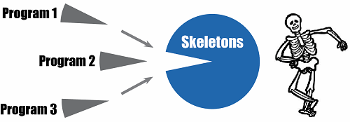
Algorithmic Skeletons offer a solution; by abstracting common patterns of communication, they allow libraries and language authors to provide robust parallel implementations which allow users to focus on solving problems, rather than having to micro-manage the tricky coordination of parallel resources. That’s all well and good, but if you said to me “Chris, surely you could illustrate this point better using a cartoon skeleton doing a jig”, I’d be inclined to agree with you.
So you take your new-found knowledge of Algorithmic Skeletons and apply it to your Mandelbrot problem. You realise that calculating each pixel is just a Map operation, so, armed with a Map skeleton, you go back to your sequential Mandelbrot code and make the necessary adjustments to use Skeletons. Now you have a program which looks just like your sequential version, but harnesses all the power of the GPU to provide near-“hand tuned” levels of performance.
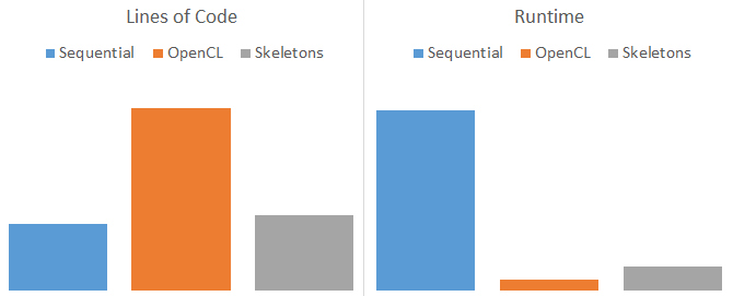
I say near hand tuned performance because clearly it’s not quite as fast as when you did all of that OpenCL programming yourself. Why is that? The reason is that by their nature, Algorithmic Skeletons are forced to forgo low-level tuning in order to generalise for all cases. If you think how hard it is to select the effective optimisations for a program, imagine trying to achieve that at the level of a patterns library for all possible use-cases! For this reason, I would argue that if we want to achieve both the of ease of use of skeletons and the high performance of hand tuned code, we need autotuning.
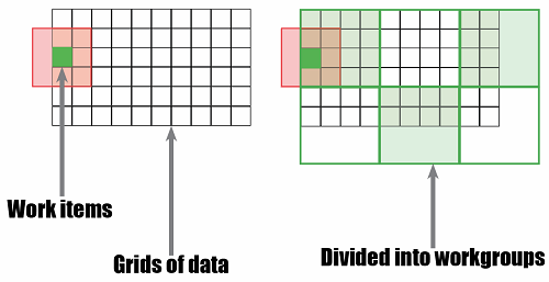
I’m going to demonstrate this argument using SkelCL, a library for Algorithmic Skeletons which targets multi-GPU systems. In particular, we’re going to focus solely on the Stencil skeleton. Stencils are patterns of computation which operate on uniform grids of data, where the value of each cell is updated based on its current value and the value of one or more neighbouring elements, which we’ll call the border region. In SkelCL, users provide the function which updates a cell’s value, and SkelCL orchestrates the parallel execution of these functions. Each cell maps to a single work item; and this collection of work items is then divided into workgroups for execution on the target hardware.
While the user is clearly in control of the type of work which is executed, the size of the grid, and the size of the border region, it is very much the responsibility of the skeleton implementation to select what workgroup size to use. As such I designed an experiment to explore just what effect changing workgroup sizes has on the performance of Stencil skeletons.
I created a set of testing workloads using 14 synthetic benchmarks representative of typical stencil applications. A selection of different dataset sizes and data types were then used to collect runtime data from 10 different combinations of CPUs, GPUs, and multi-GPUs setups.
By collecting multiple runs of each program/hardware/dataset combination using different workgroup sizes, I am able to perform relative performance comparisons to see what the best workgroup size for that combination is. By trying a bunch of different workloads and plotting the density of optimal parameter values across the space, I can start to get a feel for the optimisation space. In an ideal world, I would hope that the optimal workgroup size was the same for all workloads, i.e. that it was independent of the type of work being carried out. The ugly face of reality shows something very different.
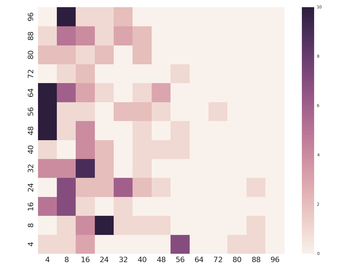
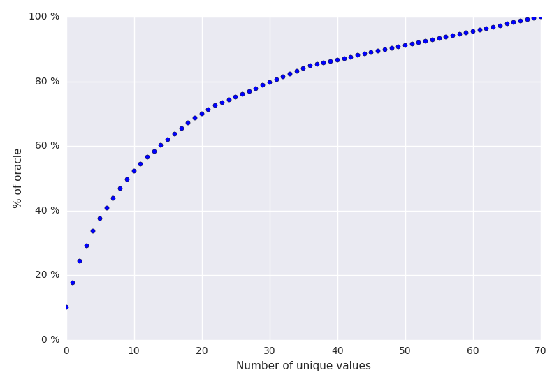
There is clearly no silver bullet value which works well for all programs, devices, and datasets. Furthermore, the values which are optimal are distributed wildly across the parameter space. By sorting the workgroup sizes by the frequency at which they were optimal, we can see that by using a fixed workgroup size, you will be optimal for only 10% of the time, at best. In fact, you need to select from 10 different workgroup sizes just to be optimal 50% of the time.
In addition, the parameter space has hard constraints. Each OpenCL device imposes a maximum workgroup size which can be checked statically. More troubling, each kernel too imposes a maximum workgroup size which can only be checked at runtime once a kernel has been compiled.
By applying these constraint tests, we can cull the list of possible workgroup sizes to generate a ZeroR powered autotuner, i.e. a simple “auto”tuner that simply selects the workgroup size that provides the highest average case performance and is legal for all cases. We can now compare speedup of all tested workgroup sizes relative to this ZeroR autotuner.
Hmm. It seems that there is a lot of room for improvement, which demonstrates the problem with having to generalise for all cases - you lose out on up to 10x performance improvements. Let’s put this all together:
- The best workgroup size for a particular workload depends on the hardware, software, and dataset.
- Not all workgroup sizes are legal, and we can only test if a value is legal at runtime.
- Differing workloads have wildly different optimal workgroup sizes, and selecting the right one can give you a 10x boost in performance.
This presents a compelling case for the development of an autotuner which can select the optimal workgroup size at runtime. That is what I have set out to achieve.
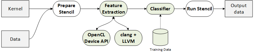
The first step to developing the autotuner is feature extraction. That means mining the dataset to begin to correlate the measured dependent variable (in this case, some measure of performance) with explanatory variables, or features. There are three sets of features we are interested in: the hardware, software, and dataset.
For hardware features, it’s simply a case of querying the OpenCL API to fetch relevant device information, such as the number of cores available, and size of local memory. Since SkelCL supports multi-GPU parallelism, we’ll make a note of how many devices were used, too.
The software features are a little more tricky. We’re looking for a way to capture some description of the computation of a given source code. For this, I first compile a kernel to LLVM bitcode, and then use the static instruction counts generated by LLVM’s InstCount to generate a feature vector of the total instruction count and the density of different kinds of instructions, e.g. the number of floating point additions per instruction. This is sufficient for my needs but it is worth noting that such a crude metric may likely fall down in the presence of sufficiently diverging control flow, since the static instruction counts would no longer resemble the number of instructions actually executed.
Dataset features are simple by comparison - I merely record the width and height of the grid, and use C++ template functions to stringify the input and output data types.
Once we have features, we can create a dataset from which will can train a machine learning classifier. We label each feature vector with the size of the workgroup that gave the best performance.
We now insert an autotuner into SkelCL which performs runtime feature extraction and classification before every stencil invocation.
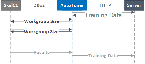
The implementation of this autotuner uses a three-tier client-server model. A master server stores the labelled training data in a common location. Then, for each SkelCL-capable machine, a system-level daemon hosts a DBus session bus which SkelCL processes can communicate with to request workgroup sizes. On launch, this daemon requests the latest training data from the master server. When a SkelCL stencil is invoked, it synchronously calls the RequestParamValues() method of the autotuner daemon, passing as arguments the required data in order to assemble a feature vector. Feature extraction then occurs within the daemon, which classifies the datapoint and returns the suggested workgroup size to the SkelCL process. This is a very low latency operation, and the system daemon can handle multiple connections from separate SkelCL processes simultaneously (although this is an admittedly unlikely use-case given that most GPGPU programs expect to be run in isolation).
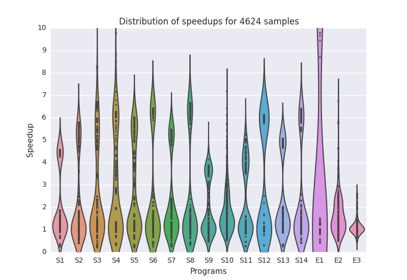
So how well does the system perform? To evaluate this, the autotuner was trained on the data collected from the synthetic benchmarks, and then tested on multiple architectures with three real world stencil applications taken from image processing, cellular automata, and a PDE solver. The runtime of the stencil using the workgroup size suggested by the autotuner was then compared against the the runtime using the best statically chosen workgroup size in order to provide some measure of speedupq.
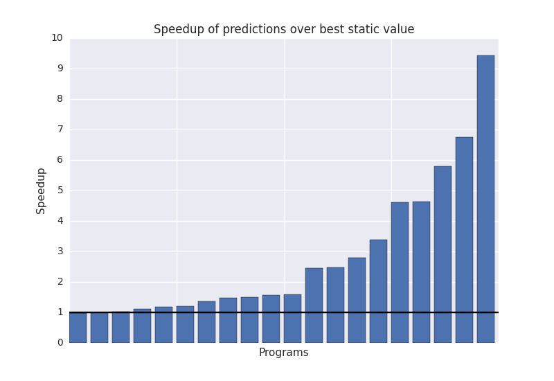
So what this shows is that using synthetic benchmarks, runtime feature extraction, and machine learning, we can improve the performance of unseen SkelCL stencil codes by an average of 2.8x.
One as yet under-explored area of this project is the feedback loop that exists when SkelCL programs are allowed to submit new datapoints to the dataset after execution with a given workgroup size has completed. While implemented, this feature is used only for collecting offline training data, and is not used for a runtime exploration of the optimisation space. More on that to come!